FE507 – Seeing Theory

Basic Probability

An introduction to the basic concepts of probability theory.

Chance Events

Randomness is all around us. Probability theory is the mathematical framework that allows us to analyze chance events in a logically sound manner. The probability of an event is a number indicating how likely that event will occur. This number is always between 0 and 1, where 0 indicates impossibility and 1 indicates certainty.

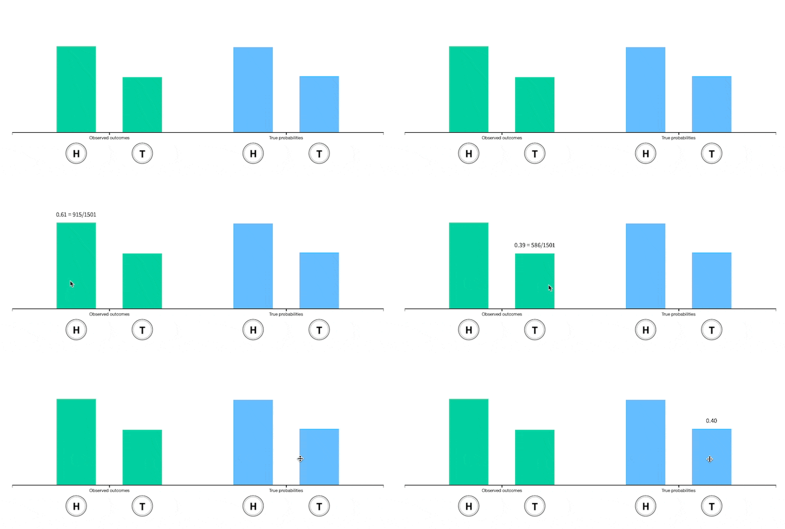
A classic example of a probabilistic experiment is a fair coin toss, in which the two possible outcomes are heads or tails. In this case, the probability of flipping a head or a tail is 1/2. In an actual series of coin tosses, we may get more or less than exactly 50% heads. But as the number of flips increases, the long-run frequency of heads is bound to get closer and closer to 50%.

CleanShot 2022-10-31 at 21.40.34

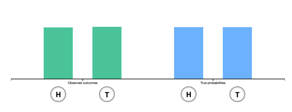
Unfair coin

CleanShot 2022-10-31 at 21.51.31

Expectation

The expectation of a random variable is a number that attempts to capture the center of that random variable's distribution.

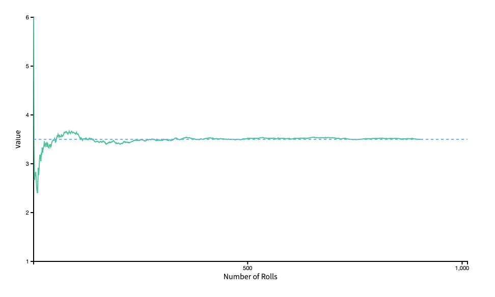
It can be interpreted as the long-run average of many independent samples from the given distribution.

More precisely, it is defined as the probability-weighted sum of all possible values in the random variable's support,

E [X] = \sum_{x \in X} x P (x)

Consider the probabilistic experiment of rolling a fair die and watch as the running sample mean converges to the expectation of 3.5.

Notice: Currrently, this is a fair die and probability for all number being got is

P (x) = 1 / 6 \approx 0.17

CleanShot 2022-10-31 at 21.47.15

CleanShot 2022-10-31 at 21.43.32

E [x] = 1 \times \frac{1}{6} + 2 \times \frac{1}{6} + 3 \times \frac{1}{6} + 4 \times \frac{1}{6} + 5 \times \frac{1}{6} + 6 \times \frac{1}{6} = \frac{21}{6} = 3.5

unfair dir

Change the distribution of the different faces of the die (thus making the die biased or "unfair") and observe how this changes the expectation.

CleanShot 2022-10-31 at 21.52.51

CleanShot 2022-10-31 at 21.58.50

E [x] = 1 \times 0.2 + 2 \times 0.16 + 3 \times 0.16 + 4 \times 0.16 + 5 \times 0.16 + 6 \times 0.16 = 0.2 + (2 + 3 + 4 + 5 + 6) \times 0.16 = 3.4

Variance

Whereas expectation provides a measure of centrality, the variance of a random variable quantifies the spread of that random variable's distribution. The variance is the average value of the squared difference between the random variable and its expectation,

Var (X) = E [(X - E [X])^{2}]

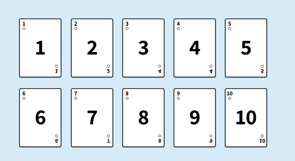
Draw cards randomly from a deck of ten cards. As you continue drawing cards, observe that the running average of squared differences (in green) begins to resemble the true variance (in blue).

E (X) = \frac{1 + 2 + 3 + 4 + 5 + 6 + 7 + 8 + 9 + 10}{10} = 55 / 10 = 5.5

Card Number	abs(X-E[X])	(X-E[X])^2	P(X)
1	4.5	20.25	1/10 = 0.1
2	3.5	12.25	0.1
3	2.5	6.25	0.1
4	1.5	2.25	0.1
5	0.5	0.25	0.1
6	0.5	0.25	0.1
7	1.5	2.25	0.1
8	2.5	6.25	0.1
9	3.5	12.25	0.1
10	4.5	20.25	0.1

V a r (X) = \frac{20.25 + 12.25 + 6.25 + 2.25 + 0.25 + 0.25 + 2.25 + 6.25 + 12.25 + 20.25}{10} = 8.25

CleanShot 2022-10-31 at 22.55.07

CleanShot 2022-10-31 at 22.55.13

Compound Probability

This chapter discusses further concepts that lie at the core of probability theory.

Set Theory

A set, broadly defined, is a collection of objects. In the context of probability theory, we use set notation to specify compound events. For example, we can represent the event "roll an even number" by the set {2, 4, 6}. For this reason it is important to be familiar with the algebra of sets.

CleanShot 2022-11-01 at 09.58.34

CleanShot 2022-11-01 at 09.58.54

CleanShot 2022-11-01 at 09.59.10

CleanShot 2022-11-01 at 10.00.05

CleanShot 2022-11-01 at 10.00.26

Counting

It can be surprisingly difficult to count the number of sequences or sets satisfying certain conditions. For example, consider a bag of marbles in which each marble is a different color. If we draw marbles one at a time from the bag without replacement, how many different ordered sequences (permutations) of the marbles are possible? How many different unordered sets (combinations)?

Permutation :

n \to P n, r

Combination:

n \to C n, r

1 marbel

CleanShot 2022-11-01 at 10.04.31

Permutation:

CleanShot 2022-11-01 at 10.03.52

Combination:

CleanShot 2022-11-01 at 10.03.52

2 marbels

CleanShot 2022-11-01 at 10.04.47

Permutation:

CleanShot 2022-11-01 at 10.05.37

Combination:

CleanShot 2022-11-01 at 10.06.19

3 marbles

CleanShot 2022-11-01 at 10.09.51

Permutation:

CleanShot 2022-11-01 at 10.07.23

Combination:

CleanShot 2022-11-01 at 10.07.55

4 marbles

CleanShot 2022-11-01 at 10.10.01

Permutation (24)

CleanShot 2022-11-01 at 10.08.32

CleanShot 2022-11-01 at 10.11.32

Combination

CleanShot 2022-11-01 at 10.08.45

CleanShot 2022-11-01 at 10.11.45

Conditional Probability

Conditional probabilities allow us to account for information we have about our system of interest. For example, we might expect the probability that it will rain tomorrow (in general) to be smaller than the probability it will rain tomorrow given that it is cloudy today. This latter probability is a conditional probability, since it accounts for relevant information that we possess.

Mathematically, computing a conditional probability amounts to shrinking our sample space to a particular event. So in our rain example, instead of looking at how often it rains on any day in general, we "pretend" that our sample space consists of only those days for which the previous day was cloudy. We then determine how many of those days were rainy.

Click on the tabs below to visualize the shrinking of the sample space.

CleanShot 2022-11-01 at 10.13.51

CleanShot 2022-11-01 at 10.14.14

CleanShot 2022-11-01 at 10.15.20

CleanShot 2022-11-01 at 10.15.34

Probability Distributions

A probability distribution specifies the relative likelihoods of all possible outcomes.

Random Variable

Formally, a random variable is a function that assigns a real number to each outcome in the probability space. Define your own discrete random variable for the uniform probability space on the right and sample to find the empirical distribution.

CleanShot 2022-11-01 at 10.21.49

Sample from probability space to generate the empirical distribution of your random variable.

CleanShot 2022-11-01 at 10.21.59

Discrete and Continues

There are two major classes of probability distributions:

Descrite
Continuous

Discrete

A discrete random variable has a finite or countable number of possible values.

CleanShot 2022-11-01 at 10.24.18

\begin{matrix} P (X = x) = f (x) \\ P (X < x) = F (X) \end{matrix}

Choose one of the following major discrete distributions to visualize. The probability mass function f(x) is shown in yellow and the cumulative distribution function F(x) in orange (controlled by the slider).

Bernoulli

A Bernoulli random variable takes the value 1 with probability of pp and the value 0 with probability of 1−p1−p. It is frequently used to represent binary experiments, such as a coin toss.

CleanShot 2022-11-01 at 10.27.23

\begin{matrix} f (x; p) = {\begin{cases} p & if x = 1 \\ 1 - p & if x = 0 \end{cases} \end{matrix}

CleanShot 2022-11-01 at 10.27.33

Binomial

A binomial random variable is the sum of nn independent Bernoulli random variables with parameter pp. It is frequently used to model the number of successes in a specified number of identical binary experiments, such as the number of heads in five coin tosses.

CleanShot 2022-11-01 at 10.28.51

CleanShot 2022-11-01 at 10.28.58

Geometric

A geometric random variable counts the number of trials that are required to observe a single success, where each trial is independent and has success probability p. For example, this distribution can be used to model the number of times a die must be rolled in order for a six to be observed.

CleanShot 2022-11-01 at 10.29.49

CleanShot 2022-11-01 at 10.29.59

Poisson

A Poisson random variable counts the number of events occurring in a fixed interval of time or space, given that these events occur with an average rate λλ. This distribution has been used to model events such as meteor showers and goals in a soccer match.

CleanShot 2022-11-01 at 10.30.36

CleanShot 2022-11-01 at 10.30.47

Negative Binomial

A negative binomial random variable counts the number of successes in a sequence of independent Bernoulli trials with parameter pp before rr failures occur. For example, this distribution could be used to model the number of heads that are flipped before three tails are observed in a sequence of coin tosses.

CleanShot 2022-11-01 at 10.31.22

CleanShot 2022-11-01 at 10.31.30

Continuous

A continuous random variable takes on an uncountably infinite number of possible values (e.g. all real numbers).

If X is a continuous random variable, then there exists unique nonnegative functions, f(x) and F(x), such that the following are true:

\begin{aligned} P (a \leq X \leq b) & = \int_{a}^{b} f (x) d x \\ P (X < x) & = F (x) \end{aligned}

CleanShot 2022-11-01 at 10.32.40

Uniform

The uniform distribution is a continuous distribution such that all intervals of equal length on the distribution's support have equal probability. For example, this distribution might be used to model people's full birth dates, where it is assumed that all times in the calendar year are equally likely.

CleanShot 2022-11-01 at 10.33.31

CleanShot 2022-11-01 at 10.33.41

Normal

The normal (or Gaussian) distribution has a bell-shaped density function and is used in the sciences to represent real-valued random variables that are assumed to be additively produced by many small effects. For example the normal distribution is used to model people's height, since height can be assumed to be the result of many small genetic and evironmental factors.

CleanShot 2022-11-01 at 10.34.23

CleanShot 2022-11-01 at 10.34.31

Student T

Student's t-distribution, or simply the t-distribution, arises when estimating the mean of a normally distributed population in situations where the sample size is small and population standard deviation is unknown.

CleanShot 2022-11-01 at 10.35.06

CleanShot 2022-11-01 at 10.35.15

Chi Squared

A chi-squared random variable with kk degrees of freedom is the sum of kkindependent and identically distributed squared standard normal random variables. It is often used in hypothesis testing and in the construction of confidence intervals.

CleanShot 2022-11-01 at 10.35.42

CleanShot 2022-11-01 at 10.35.51

FE507 – Seeing Theory

Basic Probability

Chance Events

Expectation

Variance

Compound Probability

Set Theory

Counting

3 marbles

Conditional Probability

Probability Distributions

Random Variable

Discrete and Continues

Discrete

Bernoulli

Binomial

Geometric

Poisson

Negative Binomial

Continuous

Uniform

Normal

Student T

Chi Squared

Central Limit Theorem